Your GROUP BY is lying to you: 5 window functions that reveal the truth

Every week, an analytics engineer somewhere ships a dashboard showing an Average Order Value of $150. Their CEO makes decisions based on it. Their median order is $43. Window functions would have caught this in one query. This article shows you exactly how.

As an Analytics Engineer working with e-commerce data, I see the same mistake repeated constantly: analysts aggressively GROUP BY their data to find insights, effectively discarding the row-level context that makes those insights actionable.

The pattern looks like this — you want to know your top customers, so you collapse 10,000 orders into 500 customer rows. You lose the purchase sequence. You lose the time gaps. You lose the ability to say why a customer is in the top quartile, not just that they are.

Window functions are the antidote. They let you perform sophisticated calculations — revenue rankings, cumulative distributions, moving comparisons — while keeping every individual order row intact.

This article is a focused masterclass on five functions that cover 90% of real-world analytics engineering use cases: NTILE, CUME_DIST, PERCENT_RANK, LAG/LEAD, and BigQuery's performance secret weapon, APPROX_QUANTILES.

Note on the dataset: All examples run on a synthetic e-commerce dataset.

A Quick Reminder: How window functions work

Before diving in, the mental model that makes everything click:

FUNCTION_NAME() OVER (
    PARTITION BY column_to_group_by   -- optional: defines the "window"
    ORDER BY column_to_rank_by        -- defines the ordering within the window
)

The key difference from GROUP BY: your result set keeps all original rows. The function looks across the window to compute a value, then attaches it back to each row. No collapsing. No information loss.

When to use which function: Decision tree

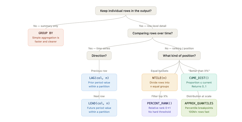
The short version:

• Need to keep individual rows? → Window function territory
• Comparing across time within a partition? → LAG / LEAD
• Ranking or positioning within a distribution?
• Equal buckets → NTILE(n)
• “Better than X% of rows” → CUME_DIST()
• Filter top X% without hard-coded thresholds → PERCENT_RANK()
• Fast distribution stats at scale → APPROX_QUANTILES
• Only need summary metrics? → GROUP BY + simple aggregation is faster and clearer

1. NTILE(4): Instant customer segmentation

The concept

NTILE(n) divides your dataset into n approximately equal buckets based on an ordering. In e-commerce, NTILE(4) gives you quartiles — the fastest path from raw order data to a segmented audience, with no clustering algorithm required.

The code

SELECT
    order_id,
    customer_name,
    product_name,
    final_amount,
    NTILE(4) OVER (
      ORDER BY final_amount DESC, order_id ASC   -- order_id as tie-breaker = deterministic
    ) AS revenue_quartile
FROM `your-project.dataset.shopify_orders`
WHERE order_status = 'completed'
ORDER BY final_amount DESC, order_id ASC
LIMIT 10

Note: ORDER BY final_amount DESC, order_id ASC is deliberate. NTILE is non-deterministic when two rows share the same final_amount — adding order_id as a tie-breaker guarantees the same output on every run.

Output

The insight

Two things stand out immediately from the real data:

Product concentration: Q1 is entirely Webcam 4K. This is not a bug — it’s a signal. Your highest-value orders are concentrated in a single SKU. A simple GROUP BY on revenue would have told you Webcam 4K is your top product, but it wouldn't have told you it dominates your entire top quartile.

Ties: $207.99, $191.99, and $175.99 each appear multiple times. Without order_id ASC as a secondary sort, BigQuery's assignment of tied rows to buckets is non-deterministic — you'd get different results on different runs.

Practical action: Design your retention campaigns by quartile. Q1 gets a white-glove loyalty program. Q4 gets a reactivation offer. The quartile boundary adapts automatically as your business grows — no hard-coded dollar thresholds to maintain.

⚠️ Caveat: NTILE distributes rows as evenly as possible, but with ties the bucket boundaries may not fall exactly where you expect. For threshold-based segmentation that must be stable across time periods, use APPROX_QUANTILES (section 5) to extract the actual dollar breakpoints first.

2. CUME_DIST(): Proportional position analysis

The concept

CUME_DIST() returns a value between 0 and 1 representing the proportion of rows with a value less than or equal to the current row's value. It answers: "What percentage of my orders is this order better than?"

Unlike a rank (an integer that depends on dataset size), CUME_DIST gives a scale-invariant position — useful when comparing distributions across time periods or customer segments of different sizes. "Was this order in the top 20% in Q1 and in Q2?" works reliably with CUME_DIST even if Q1 had 800 orders and Q2 had 1,200.

The code

SELECT
    order_id,
    customer_name,
    final_amount,
    ROUND(CUME_DIST() OVER (ORDER BY final_amount ASC), 4) AS percentile_position
FROM `your-project.dataset.shopify_orders`
WHERE order_status = 'completed'
ORDER BY final_amount DESC
LIMIT 10;

Output

The insight

All four $207.99 orders share CUME_DIST = 1.0000 — they're at the very top of the distribution. The four $191.99 orders share 0.9692, meaning they exceed ~97% of all completed orders.

On ties: Tied rows always share the highest CUME_DIST value in the group. This is mathematically correct but worth flagging to stakeholders.

Practical action: Use this to build dynamic pricing tiers. Instead of hard-coding “premium = above $180”, write WHERE percentile_position >= 0.95 — your threshold adjusts automatically as the order distribution shifts over time.

3. PERCENT_RANK(): Filtering your top X%

The concept

PERCENT_RANK() assigns a rank between 0 and 1 representing where a value sits in the ordered distribution. The formula is:

(rank - 1) / (total_rows - 1)

The key practical difference from CUME_DIST:

• PERCENT_RANK starts at 0 — the lowest value is always 0
• CUME_DIST ends at 1 — the highest value is always 1

This makes PERCENT_RANK more intuitive for "top X%" filtering: a value of 0.0 unambiguously means rank #1.

The code

SELECT
    order_id,
    customer_name,
    final_amount,
    ROUND(PERCENT_RANK() OVER (ORDER BY final_amount DESC), 4) AS pct_rank
FROM `your-project.dataset.shopify_orders`
WHERE order_status = 'completed'
ORDER BY final_amount DESC
LIMIT 10;

Output

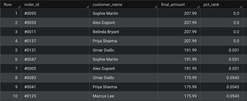
The insight

All four top-priced orders ($207.99) get pct_rank = 0.0000 — they're at rank #1. The next tier ($191.99) gets 0.031, meaning they're in the top 3% of orders.

Practical action: Wrap this in a CTE to isolate your top decile without hard-coding dollar amounts:

WITH ranked AS (
    SELECT
        order_id,
        customer_name,
        final_amount,
        PERCENT_RANK() OVER (ORDER BY final_amount DESC) AS pct_rank
    FROM `your-project.dataset.shopify_orders`
    WHERE order_status = 'completed'
)
SELECT * FROM ranked
WHERE pct_rank <= 0.10;  -- top 10% of orders, regardless of scale

This query works identically whether you have 130 or 130,000,000 orders. No threshold maintenance needed.

4. LAG() and LEAD(): Period-over-Period comparison without self-joins

The concept

LAG(col, n) accesses the value of col from n rows before the current row. LEAD(col, n) accesses n rows after. Both operate within the window defined by PARTITION BY and ORDER BY.

This is the canonical replacement for the self-join anti-pattern:

-- ❌ The self-join: slow, verbose, and fragile at scale
SELECT a.order_date, a.final_amount, b.final_amount AS prev_amount
FROM orders a
LEFT JOIN orders b
    ON a.customer_name = b.customer_name
    AND b.order_date = (
        SELECT MAX(order_date) FROM orders
        WHERE customer_name = a.customer_name
          AND order_date < a.order_date
    );

-- ✅ LAG: clean, readable, significantly faster at scale
SELECT
    order_date,
    customer_name,
    final_amount,
    LAG(final_amount, 1) OVER (
        PARTITION BY customer_name
        ORDER BY order_date
    ) AS previous_order_amount,
    final_amount - LAG(final_amount, 1) OVER (
        PARTITION BY customer_name
        ORDER BY order_date
    ) AS amount_change
FROM `your-project.dataset.shopify_orders`
WHERE order_status = 'completed'
ORDER BY customer_name, order_date;

Output

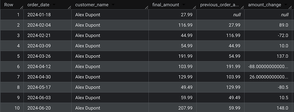
The insight

PARTITION BY customer_name is what makes this powerful: LAG resets for each customer, so you're always comparing an order to that customer's own previous purchase — never to another customer's order.

On NULLs: The first order per customer correctly returns NULL for previous_order_amount. Do not replace this with COALESCE(..., 0) — a delta of $0 is semantically incorrect. It implies no change in spend, when in reality there is no prior reference. The right production pattern is to surface NULL and handle it downstream:

-- ✅ Preferred pattern in dbt
LAG(final_amount, 1) OVER (
    PARTITION BY customer_name
    ORDER BY order_date
) AS previous_order_amount,

5. APPROX_QUANTILES: Fast Percentile Calculation at Scale

The concept

APPROX_QUANTILES is BigQuery's approximate quantile function. It computes percentile breakpoints across your entire dataset using a streaming algorithm — no window frame, no row-by-row ordering required.

This is not a traditional window function, but it belongs in every analytics engineer’s toolkit because it solves a problem that window functions handle poorly at scale: computing distribution statistics on hundreds of millions of rows.

The code

SELECT
    -- APPROX_QUANTILES(col, n) returns an array of n+1 boundary values:
    -- OFFSET(0) = min | OFFSET(1) = Q1 | OFFSET(2) = median | OFFSET(3) = Q3 | OFFSET(4) = max
    APPROX_QUANTILES(final_amount, 4)[OFFSET(1)] AS q1_threshold,
    APPROX_QUANTILES(final_amount, 4)[OFFSET(2)] AS median_value,
    APPROX_QUANTILES(final_amount, 4)[OFFSET(3)] AS q3_threshold,
    ROUND(AVG(final_amount), 2)                  AS mean_value
FROM `your-project.dataset.shopify_orders`
WHERE order_status = 'completed';

Output

The insight

The mean vs. median gap is your most important data quality signal. In this dataset, a mean of $91.53 vs. a median of $87.99 is relatively close — the distribution is not heavily skewed. But in real e-commerce data, it's common to see a mean of $150 and a median of $43, meaning a handful of high-value orders are masking typical customer behavior. Every product decision built on AOV in that scenario is distorted.

Array indexing: APPROX_QUANTILES(col, 4) returns 5 values — the minimum plus the 4 bucket boundaries. OFFSET(0) is the minimum, OFFSET(4) is the maximum. OFFSET(2) is the median. Getting this wrong is the most common error with this function.

Performance: According to the BigQuery documentation, approximate aggregate functions can be 10–100x faster than exact equivalents on large datasets, with error margins typically below 1%. On smaller datasets the gap is negligible — use PERCENTILE_CONT if you need exact values and can afford the cost.

Combine with a CASE WHEN for robust segmentation:

WITH thresholds AS (
    SELECT
        APPROX_QUANTILES(final_amount, 4)[OFFSET(1)] AS q1,
        APPROX_QUANTILES(final_amount, 4)[OFFSET(2)] AS q2,
        APPROX_QUANTILES(final_amount, 4)[OFFSET(3)] AS q3
    FROM `your-project.dataset.shopify_orders`
    WHERE order_status = 'completed'
)
SELECT
    o.order_id,
    o.customer_name,
    o.final_amount,
    CASE
        WHEN o.final_amount >= t.q3 THEN 'High Value'
        WHEN o.final_amount >= t.q2 THEN 'Mid-High'
        WHEN o.final_amount >= t.q1 THEN 'Mid-Low'
        ELSE 'Low Value'
    END AS value_segment
FROM `your-project.dataset.shopify_orders` o
CROSS JOIN thresholds t
WHERE o.order_status = 'completed';

This pattern produces stable, data-driven thresholds you can reuse consistently across dbt models — no magic numbers, no manual recalibration.

When NOT to Use Window Functions

Window functions are powerful, but they’re not always the right tool. Use simple aggregates when:

• You only need summary metrics with no row-level detail
• Your downstream BI tool (Looker, Tableau) will re-aggregate the results anyway
• You’re computing a single scalar for a dashboard KPI card

-- ❌ Overkill: window function when GROUP BY suffices
SELECT DISTINCT
    product_name,
    SUM(final_amount) OVER (PARTITION BY product_name) AS total_revenue
FROM `your-project.dataset.shopify_orders`;

-- ✅ Simpler, faster, and clearer in intent
SELECT
    product_name,
    SUM(final_amount) AS total_revenue
FROM `your-project.dataset.shopify_orders`
GROUP BY product_name;

Key Takeaways

Window functions don’t replace aggregations — they give you a richer toolkit to choose from. The decision is simpler than it looks: if you need to keep the rows, you need a window function.

• NTILE — fast, intuitive segmentation into equal buckets. Always add a tie-breaker to ORDER BY.
• CUME_DIST — scale-invariant proportional positioning. Useful across periods of different sizes.
• PERCENT_RANK — threshold-free filtering of your top X%.
• LAG / LEAD — period-over-period comparison within a partition, without self-joins. Keep NULLs as NULLs.
• APPROX_QUANTILES — distribution statistics at the speed your pipeline actually needs. Remember: OFFSET(2) is the median, not OFFSET(1).

The most expensive analytics mistake isn’t slow SQL. It’s reporting a mean when you need a median — and building a product strategy on top of it.

I’m Camille Lebrun, a Data Consultant. I write about SQL optimization, data modeling, and analytics engineering.

Found this useful? Clap on Medium to help other analytics engineers find it. What’s the most misleading aggregation you’ve seen shipped to a stakeholder? Drop it in the comments.